

Game theory and the art of litigation strategy - Article 4
Escaping the Hobbesian Trap – the impact of aggression in litigation settlement strategy
Introduction
This article that will - with the help of game theory and a little computational modelling – consider what a litigant's optimal settlement negotiation strategy should be, specifically how aggressively they should bargain with an opponent. It will build upon the framework established in the previous trilogy of articles on this topic published last year (which can be found here, here and here) which visualised how litigation settlement works and illustrated how it can become harder to settle a case the further towards trial it progresses.
So is it better to be uncompromising and bargain aggressively or be less aggressive and pragmatic? Read on to find out more.
The Hobbesian Trap
The most well-known scenario in game theory is the Prisoner's Dilemma, where two suspects in police custody are offered the opportunity to betray the other by testifying that the other committed the crime. The irony in the scenario is that if both decide to betray the other they are both worse off than if they both stayed silent.
Less well known is the Hobbesian Trap. Imagine two nations A and B, which must both decide whether to mobilise for war. Mobilising is costly (both in resources and the heightened prospect of war) but potentially advantageous if the other nation does not mobilise (because of the resulting power differential). However, if both nations mobilise neither is happy, as both will have incurred costs and heightened the risk of war without achieving any relative advantage.
We can represent this situation using the table below (which is known as a payoff matrix) where the numbers represent the relative payoff to each nation for each possible outcome. (Nation A's payoff is shown on the left of each cell and nation B's on the right of the same cell.)
|
|
Nation B |
||
|
Mobilise |
Not Mobilise |
||
|
Nation A |
Mobilise |
-2 , -2 |
+1, -1 |
|
Not Mobilise |
-1 , +1 |
0 , 0 |
|
For the purposes of this example we assume that the costs of mobilisation (-2) are greater than the disadvantage of not being mobilised when the other nation is (-1). The corresponding advantage to being a mobilised nation dealing with a nation that is not mobilised is assumed to be (+1).
If we start from a state of affairs where neither nation is mobilised, both nations have a pay-off of zero (bottom right of the matrix). However, this state is unstable as each nation has an incentive to change its position and mobilise which – assuming the other nation does not also mobilise –takes its payoff to +1 (the bottom left and top right of the matrix). Unfortunately this 'greed' incentive can result in both nations mobilising, which results in a mutual mobilisation scenario (top left). This is the worst of all positions i.e. a Hobbesian Trap.
However, if we were to start from a position of mutual mobilisation the position resembles the game of chicken – another game theory staple. In a game of chicken two cars accelerate towards each other hoping that the other will swerve away before the cars crash; if your opponent swerves and you do not then the pay-off is high whereas if neither you nor your opponent swerves the pay-off is rather less good. In the mutual mobilisation scenario, we can think of a swerve as demobilising.
|
Sidebar – How is a Hobbesian Trap different to Prisoner's Dilemma? For those who are interested, the payoff matrix for the Hobbesian Trap is different to the Prisoner's Dilemma payoff matrix, a variant of which is shown below.
The critical difference is that in a Hobbesian Trap situation, mutual mobilisation is the worst possible outcome whereas in Prisoner's Dilemma a mutual betray situation is actually a better outcome than staying silent while the other prisoner betrays you. |
|||||||||||||
As this article progresses we will consider how these scenarios could inform our understanding of litigation settlement negotiations – but first a quick recap of the framework built up in previous articles.
Litigation settlement – a recap
In summary, the key principle underpinning settlement analysis is that by settling a case (rather than taking it to trial) collectively both the claimant and defendant save the costs that would otherwise have been incurred in bringing a matter to trial; that cost saving can potentially bridge the distance between the two parties' views of what the case is worth (i.e. the claim value x probability of success, adjusting for potential costs awards).
Previous articles introduced certain terminology which will be used again in this article but which is quickly summarised below:
- An "indifference line" represents a settlement outcome that a particular party would consider financially equivalent to their expected outcome at trial; for example if a claimant's expected award at trial was £500k they would theoretically be as happy with an award of £200k at an earlier point in the litigation if they avoided incurring £300k in legal fees to take the matter to trial unnecessarily.
- The "settlement acceptance zone" is the area below the defendant's indifference line and above the claimant's indifference line – a space where both parties can settle and achieve a better outcome than they expect at trial.
- The "rational expected settlement line" is the midpoint between the claimant and defendant indifference lines.It is the point we might expect the parties to settle at assuming equal bargaining positions.
A graphical representation of these concepts is show below:
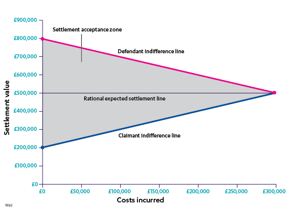
Figure 1 – Graph illustrating the claimant/defendant indifference lines, the settlement acceptance zone and the rational expected settlement line for a £1m case with a 50% chance of claimant success with both parties likely to spend £300k to take the case to trial
Litigation settlement strategy and bargaining aggression
We now have all the tools we need to start to consider what the optimal litigation settlement strategy for a lawyer to adopt might be. In this context 'settlement strategy' means the level of damages the claimant/defendant will accept/pay out and how aggressive that level is relative to the settlement acceptance zone. To do this we will consider 5 different settlement strategies below ranked on an aggression scale of 1 to 5.
|
Settlement aggression level |
Description |
|
1 |
Willing to settle at own indifference line |
|
2 |
Willing to settle midway between own indifference line and rational expected settlement line |
|
3 |
Willing to settle at the rational expected settlement line |
|
4 |
Willing to settle midway between rational expected settlement line and opponent's indifferent line |
|
5 |
Willing to settle at opponent's indifferent line |
Taking the claimant as an example, the graph below shows the point above which it would be willing to settle at different settlement aggression thresholds (please note: if the defendant's perspective were being considered Level 1 would start at the top).
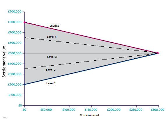
Figure 2 – The same graph as Figure 1 but with the settlement aggression levels from the Claimant's perspective shown
The caveat to the above is that one does not know what one's opponent's indifference line is as it is based on their subjective view of the prospects of success of the case. Given this limitation we will assume for the purposes of this article that a party will assess that an opponent has the same view of the prospects for the case as they do.
Measuring the outcome of a given litigation settlement strategy
To measure the effectiveness of a given strategy it is necessary to model and simulate a large number[1] of cases pitting each aggression strategy against one another.
To approximate the fact that in litigation one's knowledge and ability to accurately assess the likely outcome of the case increases over time we will split the cases into four stages where each parties level of knowledge increases at the end of each stage:
|
Litigation stage |
% Total case costs incurred by end of stage |
|
|
1 (Pleadings) |
25% |
25% |
|
2 (Own disclosure) |
50% |
50% |
|
3 (Witness statements / opponent disclosure) |
75% |
75% |
|
4 (End of trial) |
100% |
n/a as the court decides |
Each simulated case will randomly generate a claimant probability of success in the range 30%-70% (which over the spread of simulated cases means the average chance of a claimant winning a case will be 50%). We will also assume that that the claim value in all cases is £1m and each side's legal fees to trial would be £300k.
At each litigation stage the model will check whether settlement is possible – i.e. whether a settlement value exists between claimant's and defendant's bottom lines. If settlement is possible then the model will assume the parties will settle midway between their bottom lines (reflecting where we might imagine they would negotiate to)[3]. If settlement is not possible both parties progress to the next litigation stage (incurring costs as they do so). If the parties reach Stage 4 then the case is decided by the court.
Outcome of simulation
Running the numbers, the average net recovery from the claimant's perspective is as follows:
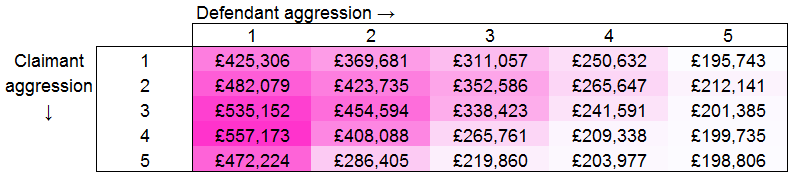
Figure 3 – Claimant average net recovery at different claimant/defendant settlement aggression levels
As one would expect, in general, the more aggressive the defendant is the lower the claimant's expected recovery for a given aggression level. This is partly due to the fact that the defendant is driving a harder bargain but also by the fact that at higher aggression levels the case is less likely to settle or if it does will settle at a later stage. This is illustrated below where the average stage the case reaches at different aggression levels is shown as a range from stage 1 (being pleadings, represented as 1.0) through to stage 4 (being trial, represented as 4.0). It can be observed that cases where one party adopts an aggression level of 5 and the other an aggression level of 4 or more do not settle.
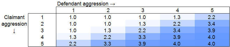
Figure 4 – Average litigation stage at which settlement is reached at different claimant/defendant settlement aggression levels
If we take Figure 3 and check what the claimant's best (vertical) response to each level of defendant aggression (along the horizontal), we get the following (with the optimal result boxed/ in bold in each case):
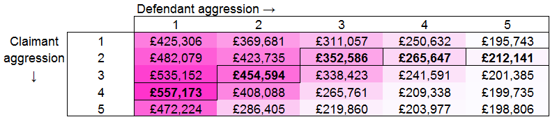
Figure 5 - Claimant average net recovery at different claimant/defendant settlement aggression levels with optimal recoveries for each defendant aggression level shown.
The same trend is reflected in the defendant's recovery graph (this time you have to consider the defendant's best horizontal response to each vertical claimant aggression level).
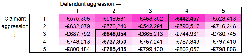
Figure 6 – Defendant average net loss at different claimant/defendant settlement aggression levels with optimal recoveries for each claimant aggression level shown.
This trend can be summarised in the table below (the result is the same regardless of whether one is claimant or defendant).
|
Opponent aggression level |
Optimal aggression level response |
|
1 |
4 |
|
2 |
3 |
|
3 |
2 |
|
4 |
2 |
|
5 |
2 |
Here we see that one's optimal aggression level depends on the aggression level of one's opponent. It is generally better to be more aggressive to a less-aggressive opponent and vice versa.
Further refinement
We can take the analysis above one step further and consider how rational adversaries will engage with this settlement landscape.
Knowing that the optimal level of aggression response to any aggression level from your opponent is in the range 2-4 there is no reason why rationally either the claimant or the defendant would adopt an aggression level of 1 or 5 so we can discount them and the table reduces to the following:
|
Opponent aggression level |
Optimal aggression level response |
|
2 |
3 |
|
3 |
2 |
|
4 |
2 |
In the reduced form we can see that the range of optimal aggression has now shrunk to 2-3. This is because level 4 is only optimal if one's opponent has aggression level 1, which we have seen they are unlikely to adopt. Eliminating level 4 from the table as well reduces the table to the following:
|
Opponent aggression level |
Optimal aggression level response |
|
2 |
3 |
|
3 |
2 |
Putting in the Claimant's expected recovery values at these levels of aggression produces the following:
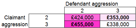
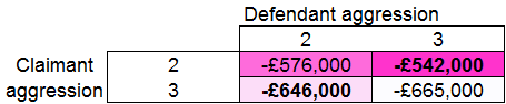
Figure 7 – Claimant average net recovery (top) and defendant average loss (bottom) at different claimant/defendant at settlement aggression levels 2 and 3 (figures rounded to nearest thousand).
By way of explanation for the table above – taking the 2/2 example – the claimant's average outcome is a recovery is £424k which reflects the fact that in those conditions it generally is able to settle at the end of litigation stage 1 (after which c. £75k costs have been incurred) for an average settlement of £500k. Similarly the defendant's average outcome is loss of -£576k (i.e. the £500k average settlement plus c. £75k of costs).
Here we come full circle if we return to our Hobbesian Trap example and think of aggression level 3 as being the equivalent of mobilising and aggression level 2 as being not mobilising. As can be seen from Figure 7, a level 2 / level 2 (demobilised) scenario is much better for both claimant and defendant than a level 3 / level 3 (mobilised) scenario. Here the desire to be more aggressive and hold out for a better deal conspires to produce a worse result (for both sides) than if both sides were less aggressive. In fact, the negative of this is more acute than in the original Hobbesian Trap scenario as the potential gain from being aggressive is small (c. £15k – £30k) relative to the cost of a level 3 / level 3 scenario (c. £90k).
Assuming a case starts from a level 3 / level 3 starting position – we are in a 'chicken like' scenario. The level 3 / level 3 starting scenario is unstable[4] because if either party lowers their aggression level to 2 (or 'swerves') the position is improved for both parties. However the hope that one's opponent will swerve first can keep both parties in the level 3 / level 3 state in which both parties – relatively speaking – lose.
Concluding thoughts
The analysis illustrates the potential dangers of adopting an overzealous approach to get the best deal for one's client. The best litigators will be able to weigh up the value of any additional concession that might be achieved against the time cost of achieving it and be mindful that too aggressive an approach could end up costing the client (much) more.
Ultimately any analysis is only as good as the underlying model which is necessarily based on a number of assumptions. However, it is hoped this article provides an alternative perspective on settlement strategy and an illustration of how to address a problem by thinking about it in a strategic context.[1] The results that follow are based on the average value of approximately 4 million simulated cases in a computer model created by RPC
[4] In the parlance of game theory – the level 2 / level 3 and level 3 / level 2 points are Nash Equilibria – were as level 3 / level 3 is not.